Electrical: Electric field

An electric field surrounds electrically charged particles and time-varying magnetic fields. The electric field depicts the surrounding force of an electrically charged particle exerted on other electrically charged objects. The concept of an electric field was introduced by Micha
el Faraday.

Qualitative description

The electric field is a vector field with SI units of newtons per coulomb (N C⁻¹) or, equivalently, volts per metre (V m⁻¹). The SI base units of the electric field are kg⋅m⋅s⁻³⋅A⁻¹. The strength or magnitude of the field at a given point is defined as the force that would be exerted on a positive test charge of 1 coulomb placed at that point; the direction of the field is given by the direction of that force. Electric fields contain electrical energy with energy density proportional to the square of the field amplitude. The electric field is to charge as gravitational acceleration is to mass and force density is to volume.
An electric field that changes with time, such as due to the motion of charged particles in the field, influences the local magnetic field. That is, the electric and magnetic fields are not completely separate phenomena; what one observer perceives as an electric field, another observer in a different frame of reference perceives as a mixture of electric and magnetic fields. For this reason, one speaks of "electromagnetism" or "electromagnetic fields". In quantum electrodynamics, disturbances in the electromagnetic fields are called photons, and the energy of photons is quantized.

Quantitative definition

Electric field from a positive Q

Electric field from a negative Q

Consider a point charge q with position (x,y,z). Now suppose the charge is subject to a force F_{on q} due to other charges. Since this force varies with the position of the charge and by Coloumb's Law it is defined at all points in space, F_{on q} is a continuous function of the charge's position (x,y,z). This suggests that there is some property of the space that causes the force which is exerted on the charge q. This property is called the electric field and it is defined by

$\mathbf{E}(x,y,z)=\frac{\mathbf{F}_\text{on q}(x,y,z)}{q}$

Notice that the magnitude of the electric field has units of Force/Charge. Mathematically, the E field can be thought of as a function that associates a vector with every point in space. Each such vector's magnitude is proportional to how much force a charge at that point would "feel" if it were present and this force would have the same direction as the electric field vector at that point. It is also important to note that the electric field defined above is caused by a configuration of other electric charges. This means that the charge q in the equation above is not the charge that is creating the electric field, but rather, being acted upon by it. This definition does not give a means of computing the electric field caused by a group of charges.
From the definition, the direction of the electric field is the same as the direction of the force it would exert on a positively charged particle, and opposite the direction of the force on a negatively charged particle. Since like charges repel and opposites attract, the electric field is directed away from positive charges and towards negative charges.

Superposition

Array of discrete point charges

Electric fields satisfy the superposition principle. If more than one charge is present, the total electric field at any point is equal to the vector sum of the separate electric fields that each point charge would create in the absence of the others.

$\mathbf{E} = \sum_i \mathbf{E}_i = \mathbf{E}_1 + \mathbf{E}_2 + \mathbf{E}_3 \cdots \,\!$

The total E-field due to N point charges is simply the superposition of the E-fields due to each point charge:

$\mathbf{E} = \sum_{i=1}^N \mathbf{E}_i = \frac{1}{4\pi\varepsilon_0} \sum_{i=1}^N \frac{Q_i}{r_i^2} \mathbf{\hat{r}}_i.$

where r_i is the position of charge Q_i, $\mathbf{\hat{r}}_i$ the corresponding unit vector.

Continuum of charges

The superposition principle holds for an infinite number of infinitesimally small elements of charges – i.e. a continuous distribution of charge. The limit of the above sum is the integral:

$\mathbf{E} = \int_V d\mathbf{E} = \frac{1}{4\pi\varepsilon_0} \int_V\frac{\rho}{r^2} \mathbf{\hat{r}}\,\mathrm{d}V = \frac{1}{4\pi\varepsilon_0} \int_V\frac{\rho}{r^3} \mathbf{r}\,\mathrm{d}V \,\!$

where ρ is the charge density (the amount of charge per unit volume), and dV is the differential volume element. This integral is a volume integral over the region of the charge distribution.

The electric field at a point is equal to the negative gradient of the electric potential there, $\mathbf{E} = -\nabla \Phi$

Coulomb's law is actually a special case of Gauss's Law, a more fundamental description of the relationship between the distribution of electric charge in space and the resulting electric field. While Columb's law (as given above) is only true for stationary point charges, Gauss's law is true for all charges either in static or in motion. Gauss's law is one of Maxwell's equations governing electromagnetism.
Gauss's law allows the E-field to be calculated in terms of a continuous distribution of charge density

$\nabla \cdot \mathbf{E} = \frac{\rho}{\varepsilon _0}.$

where ∇⋅ is the divergence operator, ρ is the total charge density, including free and bound charge, in other words all the charge present in the system (per unit volume).

Electrostatic fields

Main article: Electrostatics

Electrostatic fields are E-fields which do not change with time, which happens when the charges are stationary.

Illustration of the electric field surrounding a positive (red) and a negative (blue) charge in one dimension if the right charge is changing from positive to negative

Illustration of the electric field surrounding a positive (red) and a negative (blue) charge.

The electric field at a point E(r) is equal to the negative gradient of the electric potential Φ(r), a scalar field at the same point:

$\mathbf{E} = -\nabla \Phi$

where ∇ is the gradient. This is equivalent to the force definition above, since electric potential Φ is defined by the electric potential energy U per unit (test) positive charge:

$\Phi = \frac{U}{q}$

and force is the negative of potential energy gradient:

$\mathbf{F} = - \nabla U$

If several spatially distributed charges generate such an electric potential, e.g. in a solid, an electric field gradient may also be defined.

Uniform fields

A uniform field is one in which the electric field is constant at every point. It can be approximated by placing two conducting plates parallel to each other and maintaining a voltage (potential difference) between them; it is only an approximation because of edge effects. Ignoring such effects, the equation for the magnitude of the electric field E is:

$E = - \frac{\Delta\phi}{d}$

where Δϕ is the potential difference between the plates and d is the distance separating the plates. The negative sign arises as positive charges repel, so a positive charge will experience a force away from the positively charged plate, in the opposite direction to that in which the voltage increases. In micro- and nanoapplications, for instance in relation to semiconductors, a typical magnitude of an electric field is in the order of 1 volt/µm achieved by applying a voltage of the order of 1 volt between conductors spaced 1 µm apart.

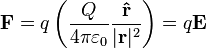
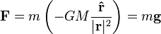
Parallels between electrostatic and gravitational fields

Electric field from a negative Q where $\mathbf{F}=q\left(\frac{Q}{4\pi\varepsilon_0}\frac{\mathbf{\hat{r}}}{|\mathbf{r}|^2}\right)=q\mathbf{E}$

Coulomb's law, which describes the interaction of electric charges:

$\mathbf{F}=q\left(\frac{Q}{4\pi\varepsilon_0}\frac{\mathbf{\hat{r}}}{|\mathbf{r}|^2}\right)=q\mathbf{E}$

is similar to Newton's law of universal gravitation:

$\mathbf{F}=m\left(-GM\frac{\mathbf{\hat{r}}}{|\mathbf{r}|^2}\right)=m\mathbf{g}$ .

This suggests similarities between the electric field E and the gravitational field g, so sometimes mass is called "gravitational charge".
Similarities between electrostatic and gravitational forces:

Both act in a vacuum.
Both are central and conservative.
Both obey an inverse-square law (both are inversely proportional to square of r).

Differences between electrostatic and gravitational forces:

Electrostatic forces are much greater than gravitational forces for natural values of charge and mass. For instance, the ratio of the electrostatic force to the gravitational force between two electrons is about 10⁴².
Gravitational forces are attractive for like charges, whereas electrostatic forces are repulsive for like charges.
There are not negative gravitational charges (no negative mass) while there are both positive and negative electric charges. This difference, combined with the previous two, implies that gravitational forces are always attractive, while electrostatic forces may be either attractive or repulsive.

Electrodynamic fields

Main article: Electrodynamics

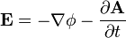
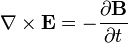
Electrodynamic fields are E-fields which do change with time, when charges are in motion.
An electric field can be produced, not only by a static charge, but also by a changing magnetic field. The electric field is given by:

$\mathbf{E} = - \nabla \phi - \frac { \partial \mathbf{A} } { \partial t }$

in which B satisfies

$\mathbf{B} = \nabla \times \mathbf{A}$

and ∇× denotes the curl. The vector field B is the magnetic flux density and the vector A is the magnetic vector potential. Taking the curl of the electric field equation we obtain,

$\nabla \times \mathbf{E} = -\frac{\partial \mathbf{B}} {\partial t}$

which is Faraday's law of induction, another one of Maxwell's equations.^[1]

Energy in the electric field

Main article: Electric potential energy

The electrostatic field stores energy. The energy density u (energy per unit volume) is given by^[2]

$u = \frac{1}{2} \varepsilon |\mathbf{E}|^2 \, ,$

where ε is the permittivity of the medium in which the field exists, and E is the electric field vector (in newtons per coulomb).
The total energy U stored in the electric field in a given volume V is therefore

$U = \frac{1}{2} \varepsilon \int_{V} |\mathbf{E}|^2 \, \mathrm{d}V \, ,$

Further extensions

Definitive equation of vector fields

In the presence of matter, it is helpful in electromagnetism to extend the notion of the electric field into three vector fields, rather than just one:^[3]

$\mathbf{D}=\varepsilon_0\mathbf{E}+\mathbf{P}\!$

where P is the electric polarization – the volume density of electric dipole moments, and D is the electric displacement field. Since E and P are defined separately, this equation can be used to define D. The physical interpretation of D is not as clear as E (effectively the field applied to the material) or P (induced field due to the dipoles in the material), but still serves as a convenient mathematical simplification, since Maxwell's equations can be simplified in terms of free charges and currents.

Constitutive relation

Main article: Constitutive equation

The E and D fields are related by the permittivity of the material, ε.^[4]^[5]
For linear, homogeneous, isotropic materials E and D are proportional and constant throughout the region, there is no position dependence: For inhomogeneous materials, there is a position dependence throughout the material:

$\mathbf{D(r)}=\varepsilon\mathbf{E(r)}$

For anisotropic materials the E and D fields are not parallel, and so E and D are related by the permittivity tensor (a 2nd order tensor field), in component form:

$D_i=\varepsilon_{ij}E_j$

For non-linear media, E and D are not proportional. Materials can have varying extents of linearity, homogeneity and isotropy.

http://en.wikipedia.org/wiki/Electric_field

Electrical

Pages

Saturday, April 27, 2013

Electric field