Electrical resistivity and conductivity

Electrical resistivity (also known as resistivity, specific electrical resistance, or volume resistivity) quantifies how strongly a given material opposes the flow of electric current. A low resistivity indicates a material that readily allows the movement of electri
c charge. Resistivity is commonly represented by the Greek letter ρ (rho). The SI unit of electrical resistivity is the ohm⋅metre (Ω⋅m)^[1][2][3] although other units like ohm⋅centimetre (Ω⋅cm) are also in use. As an example, if a 1m×1m×1m solid cube of material has sheet contacts on two opposite faces, and the resistance between these contacts is 1Ω, then the resistivity of the material is 1Ω⋅m.
Electrical conductivity or specific conductance is the reciprocal of electrical resistivity, and measures a material's ability to conduct an electric current. It is commonly represented by the Greek letter σ (sigma), but κ (kappa) (especially in electrical engineering) or γ (gamma) are also occasionally used. Its SI unit is siemens per metre (S⋅m⁻¹) and CGSE unit is reciprocal second (s⁻¹).

Definition

Resistors or conductors with uniform cross-section

A piece of resistive material with electrical contacts on both ends.

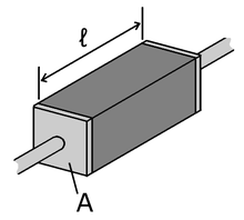
Many resistors and conductors have a uniform cross section with a uniform flow of electric current and are made of one material. (See the diagram to the right.) In this case, the electrical resistivity ρ (Greek: rho) is defined as:

where

R is the electrical resistance of a uniform specimen of the material (measured in ohms, Ω)

is the length of the piece of material (measured in metres, m)

A is the cross-sectional area of the specimen (measured in square metres, m²).

The reason resistivity is defined this way is that it makes resistivity a material property, unlike resistance. All copper wires, irrespective of their shape and size, have approximately the same resistivity, but a long, thin copper wire has a much larger resistance than a thick, short copper wire. Every material has its own characteristic resistivity – for example, rubber's resistivity is far larger than copper's.
In a hydraulic analogy, passing current through a high-resistivity material is like pushing water through a pipe full of sand, while passing current through a low-resistivity material is like pushing water through an empty pipe. If the pipes are the same size and shape, the pipe full of sand has higher resistance to flow. But resistance is not solely determined by the presence or absence of sand; it also depends on how wide the pipe is (it is harder to push water through a skinny pipe than a wide one) and how long it is (it is harder to push water through a long pipe than a short one.)
The above equation can be transposed to get Pouillet's law:

The resistance of a given material will increase with the length, but decrease with increasing cross-sectional area. From the above equations, resistivity has SI units of ohm⋅metre. Other units like ohm⋅cm or ohm⋅inch are also sometimes used.
The formula can be used to intuitively understand the meaning of a resistivity value. For example, if and (forming a cube with perfectly-conductive contacts on opposite faces), then the resistance of this element in ohms is numerically equal to the resistivity of the material it is made of in ohm-meters. Likewise, a 1 ohm⋅cm material would have a resistance of 1 ohm if contacted on opposite faces of a 1 cm×1 cm×1 cm cube.
Conductivity σ (Greek: sigma) is defined as the inverse of resistivity:

Conductivity has SI units of siemens per meter (S/m).

General definition

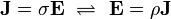
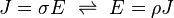
The above definition was specific to resistors or conductors with a uniform cross-section, where current flows uniformly through them. A more basic and general definition starts from the fact that if there is electric field inside a material, it will cause electric current to flow. The electrical resistivity ρ is defined as the ratio of the electric field to the density of the current it creates:

where

ρ is the resistivity of the conductor material (measured in ohm⋅metres, Ω⋅m),

E is the magnitude of the electric field (in volts per metre, V⋅m⁻¹),

J is the magnitude of the current density (in amperes per square metre, A⋅m⁻²),

in which E and J are inside the conductor.
Conductivity is the inverse:

For example, rubber is a material with large ρ and small σ, because even a very large electric field in rubber will cause almost no current to flow through it. On the other hand, copper is a material with small ρ and large σ, because even a small electric field pulls a lot of current through it.

Causes of conductivity

Band theory simplified

Electron energy levels in an insulator

Quantum mechanics states that electrons in an atom cannot take on any arbitrary energy value. Rather, there are fixed energy levels which the electrons can occupy, and values in between these levels are impossible. When a large number of such allowed energy levels are spaced close together (in energy-space) i.e. have similar (minutely differing energies) then we can talk about these energy levels together as an "energy band". There can be many such energy bands in a material, depending on the atomic number (number of electrons) and their distribution (besides external factors like environment modifying the energy bands). Two such bands important in the discussion of conductivity of materials are: the valence band and the conduction band (the latter is generally above the former)^{[citation needed]}. Electrons in the conduction band may move freely throughout the material in the presence of an electrical field.
In insulators and semiconductors, the atoms in the substance influence each other so that between the valence band and the conduction band there exists a forbidden band of energy levels, which the electrons cannot occupy. In order for a current to flow, a relatively large amount of energy must be furnished to an electron for it to leap across this forbidden gap and into the conduction band. Thus, even large voltages can yield relatively small currents.

In metals

A metal consists of a lattice of atoms, each with an outer shell of electrons which freely dissociate from their parent atoms and travel through the lattice. This is also known as a positive ionic lattice.^[4] This 'sea' of dissociable electrons allows the metal to conduct electric current. When an electrical potential difference (a voltage) is applied across the metal, the resulting electric field causes electrons to move from one end of the conductor to the other.
Near room temperatures, metals have resistance. The primary cause of this resistance is the thermal motion of ions. This acts to scatter electrons (due to destructive interference of free electron waves on non-correlating potentials of ions)^{[citation needed]}. Also contributing to resistance in metals with impurities are the resulting imperfections in the lattice. In pure metals this source is negligible^{[citation needed]}.
The larger the cross-sectional area of the conductor, the more electrons per unit length are available to carry the current. As a result, the resistance is lower in larger cross-section conductors. The number of scattering events encountered by an electron passing through a material is proportional to the length of the conductor. The longer the conductor, therefore, the higher the resistance. Different materials also affect the resistance.^[5]

In semiconductors and insulators

Main articles: Semiconductor and Insulator (electricity)

In metals, the Fermi level lies in the conduction band (see Band Theory, above) giving rise to free conduction electrons. However, in semiconductors the position of the Fermi level is within the band gap, approximately half-way between the conduction band minimum and valence band maximum for intrinsic (undoped) semiconductors. This means that at 0 kelvins, there are no free conduction electrons and the resistance is infinite. However, the resistance will continue to decrease as the charge carrier density in the conduction band increases. In extrinsic (doped) semiconductors, dopant atoms increase the majority charge carrier concentration by donating electrons to the conduction band or accepting holes in the valence band. For both types of donor or acceptor atoms, increasing the dopant density leads to a reduction in the resistance, hence highly doped semiconductors behave metallically. At very high temperatures, the contribution of thermally generated carriers will dominate over the contribution from dopant atoms and the resistance will decrease exponentially with temperature.

In ionic liquids/electrolytes

Main article: Conductivity (electrolytic)

In electrolytes, electrical conduction happens not by band electrons or holes, but by full atomic species (ions) traveling, each carrying an electrical charge. The resistivity of ionic liquids varies tremendously by the concentration – while distilled water is almost an insulator, salt water is a very efficient electrical conductor. In biological membranes, currents are carried by ionic salts. Small holes in the membranes, called ion channels, are selective to specific ions and determine the membrane resistance.

Superconductivity

Main article: Superconductivity

The electrical resistivity of a metallic conductor decreases gradually as temperature is lowered. In ordinary conductors, such as copper or silver, this decrease is limited by impurities and other defects. Even near absolute zero, a real sample of a normal conductor shows some resistance. In a superconductor, the resistance drops abruptly to zero when the material is cooled below its critical temperature. An electric current flowing in a loop of superconducting wire can persist indefinitely with no power source.^[6]
In 1986, it was discovered that some cuprate-perovskite ceramic materials have a critical temperature above 90 K (−183 °C). Such a high transition temperature is theoretically impossible for a conventional superconductor, leading the materials to be termed high-temperature superconductors. Liquid nitrogen boils at 77 K, facilitating many experiments and applications that are less practical at lower temperatures. In conventional superconductors, electrons are held together in pairs by an attraction mediated by lattice phonons. The best available model of high-temperature superconductivity is still somewhat crude. There is a hypothesis that electron pairing in high-temperature superconductors is mediated by short-range spin waves known as paramagnons.^[7]

Resistivity of various materials

Main article: Electrical resistivities of the elements (data page)

• A conductor such as a metal has high conductivity and a low resistivity.
• An insulator like glass has low conductivity and a high resistivity.
• The conductivity of a semiconductor is generally intermediate, but varies widely under different conditions, such as exposure of the material to electric fields or specific frequencies of light, and, most important, with temperature and composition of the semiconductor material.

The degree of doping in semiconductors makes a large difference in conductivity. To a point, more doping leads to higher conductivity. The conductivity of a solution of water is highly dependent on its concentration of dissolved salts, and other chemical species that ionize in the solution. Electrical conductivity of water samples is used as an indicator of how salt-free, ion-free, or impurity-free the sample is; the purer the water, the lower the conductivity (the higher the resistivity). Conductivity measurements in water are often reported as specific conductance, relative to the conductivity of pure water at 25 °C. An EC meter is normally used to measure conductivity in a solution. A rough summary is as follows:

Material	Resistivity ρ (Ω•m)
Superconductors	0
Metals	10−8
Semiconductors	variable
Electrolytes	variable
Insulators	1016

This table shows the resistivity, conductivity and temperature coefficient of various materials at 20 °C (68 °F, 293 K)

Material	ρ (Ω•m) at 20 °C	σ (S/m) at 20 °C	Temperature coefficient[note 1] (K−1)	Reference
Silver	1.59×10−8	6.30×107	0.0038	[8][9]
Copper	1.68×10−8	5.96×107	0.0068	[10]
Annealed copper[note 2]	1.72×10−8	5.80×107	0.00393	[11]
Gold[note 3]	2.44×10−8	4.10×107	0.0034	[8]
Aluminium[note 4]	2.82×10−8	3.5×107	0.0039	[8]
Calcium	3.36×10−8	2.98×107	0.0041
Tungsten	5.60×10−8	1.79×107	0.0045	[8]
Zinc	5.90×10−8	1.69×107	0.0037	[12]
Nickel	6.99×10−8	1.43×107	0.006
Lithium	9.28×10−8	1.08×107	0.006
Iron	1.0×10−7	1.00×107	0.005	[8]
Platinum	1.06×10−7	9.43×106	0.00392	[8]
Tin	1.09×10−7	9.17×106	0.0045
Carbon steel (1010)	1.43×10−7	6.99×106		[13]
Lead	2.2×10−7	4.55×106	0.0039	[8]
Titanium	4.20×10−7	2.38×106	X
Grain oriented electrical steel	4.60×10−7	2.17×106		[14]
Manganin	4.82×10−7	2.07×106	0.000002	[15]
Constantan	4.9×10−7	2.04×106	0.000008	[16]
Stainless steel[note 5]	6.9×10−7	1.45×106		[17]
Mercury	9.8×10−7	1.02×106	0.0009	[15]
Nichrome[note 6]	1.10×10−6	9.09×105	0.0004	[8]
GaAs	5×10−7 to 10×10−3	5×10−8 to 103		[18]
Carbon (amorphous)	5×10−4 to 8×10−4	1.25 to 2×103	−0.0005	[8][19]
Carbon (graphite)[note 7]	2.5e×10−6 to 5.0×10−6 //basal plane 3.0×10−3 ⊥basal plane	2 to 3×105 //basal plane 3.3×102 ⊥basal plane		[20]
Carbon (diamond)	1×1012	~10−13		[21]
Germanium[note 8]	4.6×10−1	2.17	−0.048	[8][9]
Sea water[note 9]	2×10−1	4.8		[22]
Drinking water[note 10]	2×101 to 2×103	5×10−4 to 5×10−2		[citation needed]
Silicon[note 8]	6.40×102	1.56×10−3	−0.075	[8]
Wood(damp)	1×103 to 4	10−4 to -3		[23]
Deionized water[note 11]	1.8×105	5.5×10−6		[24]
Glass	10×1010 to 10×1014	10−11 to 10−15	?	[8][9]
Hard rubber	1×1013	10−14	?	[8]
Wood(oven dry)	1×1014 to 16	10−16 to -14		[23]
Sulfur	1×1015	10−16	?	[8]
Air	1.3×1016 to 3.3×1016	3×10−15 to 8×10−15		[25]
Paraffin wax	1×1017	10−18	?
Fused quartz	7.5×1017	1.3×10−18	?	[8]
PET	10×1020	10−21	?
Teflon	10×1022 to 10×1024	10−25 to 10−23	?

The effective temperature coefficient varies with temperature and purity level of the material. The 20 °C value is only an approximation when used at other temperatures. For example, the coefficient becomes lower at higher temperatures for copper, and the value 0.00427 is commonly specified at 0 °C.^[26]
The extremely low resistivity (high conductivity) of silver is characteristic of metals. George Gamow tidily summed up the nature of the metals' dealings with electrons in his science-popularizing book, One, Two, Three...Infinity (1947): "The metallic substances differ from all other materials by the fact that the outer shells of their atoms are bound rather loosely, and often let one of their electrons go free. Thus the interior of a metal is filled up with a large number of unattached electrons that travel aimlessly around like a crowd of displaced persons. When a metal wire is subjected to electric force applied on its opposite ends, these free electrons rush in the direction of the force, thus forming what we call an electric current." More technically, the free electron model gives a basic description of electron flow in metals.
Wood is widely regarded as an extremely good insulator, but its resistivity is sensitively dependent on moisture content, with damp wood being a factor of at least 10×10²⁰ worse insulator than oven-dry.^[23] In any case, a sufficiently high voltage - such as that in lightning strikes or some high-tension powerlines - can lead to insulation breakdown and electrocution risk even with apparently dry wood.

Temperature dependence

Linear approximation

The electrical resistivity of most materials changes with temperature. If the temperature T does not vary too much, a linear approximation is typically used:

where is called the temperature coefficient of resistivity, is a fixed reference temperature (usually room temperature), and is the resistivity at temperature . The parameter is an empirical parameter fitted from measurement data. Because the linear approximation is only an approximation, is different for different reference temperatures. For this reason it is usual to specify the temperature that was measured at with a suffix, such as , and the relationship only holds in a range of temperatures around the reference.^[27] When the temperature varies over a large temperature range, the linear approximation is inadequate and a more detailed analysis and understanding should be used.

Metals

In general, electrical resistivity of metals increases with temperature. Electron–phonon interactions can play a key role. At high temperatures, the resistance of a metal increases linearly with temperature. As the temperature of a metal is reduced, the temperature dependence of resistivity follows a power law function of temperature. Mathematically the temperature dependence of the resistivity ρ of a metal is given by the Bloch–Grüneisen formula:

where is the residual resistivity due to defect scattering, A is a constant that depends on the velocity of electrons at the Fermi surface, the Debye radius and the number density of electrons in the metal. is the Debye temperature as obtained from resistivity measurements and matches very closely with the values of Debye temperature obtained from specific heat measurements. n is an integer that depends upon the nature of interaction:

1. n=5 implies that the resistance is due to scattering of electrons by phonons (as it is for simple metals)
2. n=3 implies that the resistance is due to s-d electron scattering (as is the case for transition metals)
3. n=2 implies that the resistance is due to electron–electron interaction.

If more than one source of scattering is simultaneously present, Matthiessen's Rule (first formulated by Augustus Matthiessen in the 1860s) ^[28][29] says that the total resistance can be approximated by adding up several different terms, each with the appropriate value of n.
As the temperature of the metal is sufficiently reduced (so as to 'freeze' all the phonons), the resistivity usually reaches a constant value, known as the residual resistivity. This value depends not only on the type of metal, but on its purity and thermal history. The value of the residual resistivity of a metal is decided by its impurity concentration. Some materials lose all electrical resistivity at sufficiently low temperatures, due to an effect known as superconductivity.
An investigation of the low-temperature resistivity of metals was the motivation to Heike Kamerlingh Onnes's experiments that led in 1911 to discovery of superconductivity. For details see History of superconductivity.

Semiconductors

Main article: Semiconductor

In general, resistivity of intrinsic semiconductors decreases with increasing temperature. The electrons are bumped to the conduction energy band by thermal energy, where they flow freely and in doing so leave behind holes in the valence band which also flow freely. The electric resistance of a typical intrinsic (non doped) semiconductor decreases exponentially with the temperature:

An even better approximation of the temperature dependence of the resistivity of a semiconductor is given by the Steinhart–Hart equation:

where A, B and C are the so-called Steinhart–Hart coefficients.
This equation is used to calibrate thermistors.
Extrinsic (doped) semiconductors have a far more complicated temperature profile. As temperature increases starting from absolute zero they first decrease steeply in resistance as the carriers leave the donors or acceptors. After most of the donors or acceptors have lost their carriers the resistance starts to increase again slightly due to the reducing mobility of carriers (much as in a metal). At higher temperatures it will behave like intrinsic semiconductors as the carriers from the donors/acceptors become insignificant compared to the thermally generated carriers.^[30]
In non-crystalline semiconductors, conduction can occur by charges quantum tunnelling from one localised site to another. This is known as variable range hopping and has the characteristic form of

,

where n = 2, 3, 4, depending on the dimensionality of the system.

Complex resistivity and conductivity

When analyzing the response of materials to alternating electric fields, in applications such as electrical impedance tomography,^[31] it is necessary to replace resistivity with a complex quantity called impeditivity (in analogy to electrical impedance). Impeditivity is the sum of a real component, the resistivity, and an imaginary component, the reactivity (in analogy to reactance). The magnitude of Impeditivity is the square root of sum of squares of magnitudes of resistivity and reactivity.
Conversely, in such cases the conductivity must be expressed as a complex number (or even as a matrix of complex numbers, in the case of anisotropic materials) called the admittivity. Admittivity is the sum of a real component called the conductivity and an imaginary component called the susceptivity.
An alternative description of the response to alternating currents uses a real (but frequency-dependent) conductivity, along with a real permittivity. The larger the conductivity is, the more quickly the alternating-current signal is absorbed by the material (i.e., the more opaque the material is). For details, see Mathematical descriptions of opacity.

Tensor equations for anisotropic materials

Some materials are anisotropic, meaning they have different properties in different directions. For example, a crystal of graphite consists microscopically of a stack of sheets, and current flows very easily through each sheet, but moves much less easily from one sheet to the next.^[20]
For an anisotropic material, it is not generally valid to use the scalar equations

For example, the current may not flow in exactly the same direction as the electric field. Instead, the equations are generalized to the 3D tensor form^[32][33]

where the conductivity σ and resistivity ρ are rank-2 tensors (in other words, 3×3 matrices). The equations are compactly illustrated in component form (using index notation and the summation convention):^[34]

The σ and ρ tensors are inverses (in the sense of a matrix inverse). The individual components are not necessarily inverses; for example, σ_xx may not be equal to 1/ρ_xx.

Resistance versus resistivity in complicated geometries

If the material's resistivity is known, calculating the resistance of something made from it may, in some cases, be much more complicated than the formula above. One example is Spreading Resistance Profiling, where the material is inhomogeneous (different resistivity in different places), and the exact paths of current flow are not obvious.
In cases like this, the formulas

need to be replaced with

where E and J are now vector fields. This equation, along with the continuity equation for J and the Poisson equation for E, form a set of partial differential equations. In special cases, an exact or approximate solution to these equations can be worked out by hand, but for very accurate answers in complex cases, computer methods like finite element analysis may be required.

Resistivity density products

In some applications where the weight of an item is very important resistivity density products are more important than absolute low resistivity – it is often possible to make the conductor thicker to make up for a higher resistivity; and then a low resistivity density product material (or equivalently a high conductance to density ratio) is desirable. For example, for long distance overhead power lines, aluminium is frequently used rather than copper because it is lighter for the same conductance.

Material	Resistivity (nΩ•m)	Density (g/cm3)	Resistivity-density product (nΩ•m•g/cm3)
Sodium	47.7	0.97	46
Lithium	92.8	0.53	49
Calcium	33.6	1.55	52
Potassium	72.0	0.89	64
Beryllium	35.6	1.85	66
Aluminium	26.50	2.70	72
Magnesium	43.90	1.74	76.3
Copper	16.78	8.96	150
Silver	15.87	10.49	166
Gold	22.14	19.30	427
Iron	96.1	7.874	757

Silver, although it is the least resistive metal known, has a high density and does poorly by this measure. Calcium and the alkali metals have the best resistivity-density products, but are rarely used for conductors due to their high reactivity with water and oxygen. Aluminium is far more stable. Two other important attributes, price and toxicity, exclude the (otherwise) best choice: Beryllium. Thus, aluminium is usually the metal of choice when the weight of some required conduction (and/or the cost of conduction) is the driving consideration.

                         http://en.wikipedia.org/wiki/Electrical_resistivity_and_conductivity